Compare the operating cost of importing goods with producing them on Mars. Cheap transport can help establish a settlement while making imports more attractive. Lower local cost alone does not establish manufacturing capability or independence.
MARS INDUSTRY · IMPORT OR PRODUCE
woolong.com · Physical Frontiers
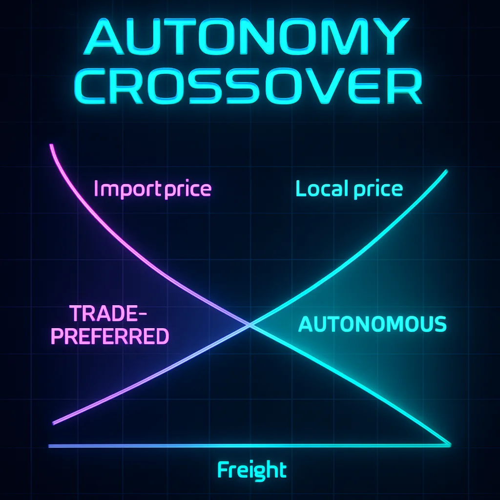
Historical illustration; “autonomy” denotes the original cost comparison. Cheaper freight → fewer goods favor local production; expensive freight → more items favor local production under these assumptions.
This tool shows how relative operating costs change as freight prices fall.
For each item it compares: (1) the landed import price from Earth and (2) the local Mars manufacturing price under your assumptions.
When freight is expensive, the model classifies more items as Local production cheaper.
As freight gets cheaper, importing becomes attractive and some items shift to Import cheaper.
Quick Start
1) Drag the transport slider. 2) Watch which rows switch between Local production cheaper and Import cheaper.
3) Edit Earth cost or equipment mass to reflect your scenario. The chart shows the unweighted share of listed goods classified as Local production cheaper at each freight price.
Global Inputs
Per-kg derived automatically.
Static in this model. Lower it manually to simulate tech/scale gains.
Spares, QA, training, downtime.
Presets:
Illustrative inputs; prices and equipment masses are not verified estimates. CSV (no header): Name, EarthCostUSDperKg, CapitalMassKG.
Sensitivity: Transport Cost
Transport (USD/ton)
300,000
Transport (USD/kg)
300.00
Mars Multiplier (×)
5.0
Overhead (%)
20%
Reading the curve: the left side is cheap freight — fewer goods favor local production.
The right side is expensive freight — more basic goods favor local production.
Y-axis: unweighted share of items that are Local production cheaper. X-axis: freight price (log scale).
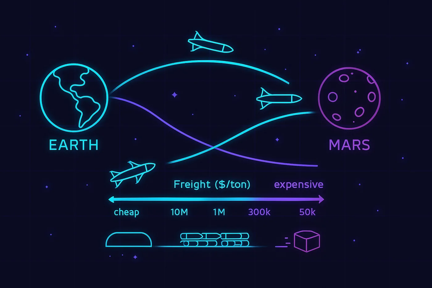
Freight slider metaphor: cheap ← → expensive.
Factory Transport Cost
Goods & Operating Cost Comparison
Edit Item, Earth Cost, or Equipment Mass.
Note: the slider only changes freight. Improvements in Mars productivity are not modeled dynamically; adjust the multiplier/overhead to test scenarios.
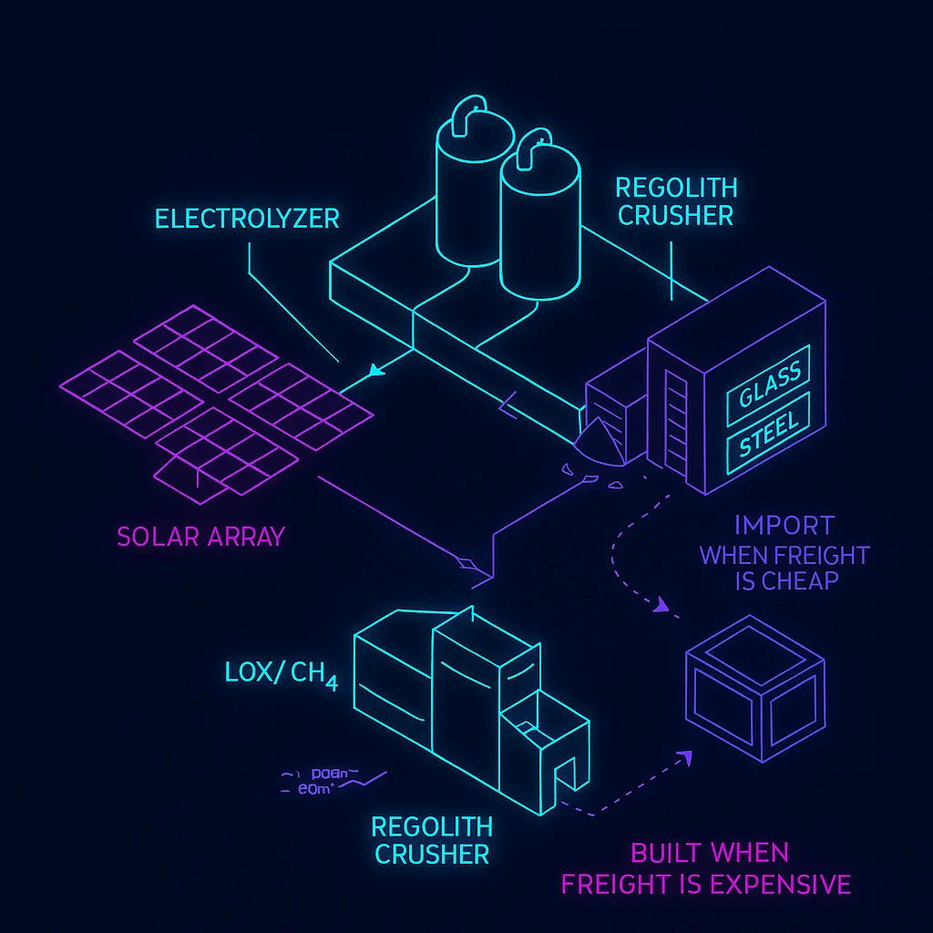
Illustrative local production cell. Relative costs alone do not establish whether it can be built.
Item
Earth Cost ($/kg)
Landed Import ($/kg)
Local Mars ($/kg)
Status
Equipment Mass (kg)
Factory Transport Cost ($)
Break-even Transport ($/ton)
Break-even Multiplier (×)
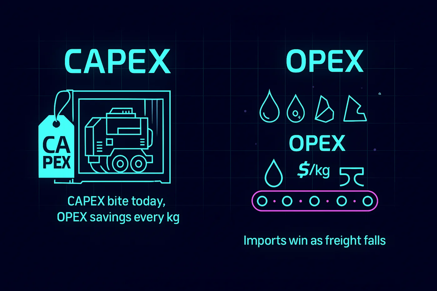
Operating vs. Capital: “Local production cheaper” compares per-kg operating costs. Factory Transport Cost shows the one-time launch bill to ship the factory. You can be operating-cheaper and still defer the build if capital is tight.
CAPEX bite today vs OPEX savings per kg; as freight falls, importing can win again.
How This Calculator Works
1) Global Inputs
Transport cost to Mars
Delivery fee per ton. The slider spans early freight (~$100M/ton) down to illustrative lower freight values (~$300k/ton) and beyond.
Mars cost multiplier (×)
How much more expensive local manufacturing is than Earth. Lower this to simulate technology, automation, and scale improvements.
Scale & complexity overhead (%)
Extra small-market penalties (spares, QA, training, downtime) applied on top of the multiplier.
2) Columns
Landed Import ($/kg)
Earth Cost + Transport/kg
Local Mars ($/kg)
Earth Cost × Multiplier × (1 + Overhead)
Status
🟢 Local production cheaper (local cheaper), 🔴 Import cheaper (import cheaper), 🟡 within ±5% Near Break-Even
Break-even Transport
Freight price where import = local, given the current multiplier.
Break-even Multiplier
Manufacturing penalty where local = import, given the current freight.
What flips first?
Bulk, low-complexity goods (water, oxygen, methane, cement, glass) — higher freight prices favor local production under the model assumptions.
What flips last?
High value-density, complex goods (electronics, precision bearings, biologics) — imports stay attractive until Mars’ multiplier improves.
Does “Local production cheaper” equal full self-sufficiency?
It is only an operating-cost comparison. Full independence also requires equipment, feedstocks, energy, and skills. Use Equipment Mass to visualize the startup cost.
What isn’t modeled dynamically?
Productivity gains on Mars. Adjust the multiplier/overhead manually to explore improved efficiency scenarios.
Historical Bebop-flavored permit: “Autonomous (High Freight)” vs “Trade-Preferred (Low Freight)”. These are the original cost-comparison labels.
What would have to be true?
The model assumes each listed good can be manufactured locally at Earth unit cost × Mars multiplier × overhead factor. The default commodity prices and factory masses are illustrative inputs without verified provenance; their precision does not imply an engineered factory design.
Factory transport cost includes only shipping the listed equipment mass. It excludes buying and installing equipment, working capital, imported feedstocks, and capital amortization. Annual demand, equipment life, local skills, supply-chain completeness, and resilience are not modeled.
The chart counts each row equally. It is not a share of total consumption, spending, or settlement self-sufficiency. Near-break-even goods are classified consistently in the table and chart using a ±5% band relative to import cost.
Historical terminology and scenarios
The original tool called lower-cost local production “Autonomous” and imports “Trade-Preferred.” Those labels described an operating-cost comparison, not proven independence. The original Pioneer, Transition, Starship Mature, and Far Future presets remain available as illustrative freight scenarios.